The previous article demonstrated the need for dynamically adjusting parameters and how to evaluate the quality of estimates by studying the order arrival intervals. This article will focus on depth data and study the mid-price (also known as fair-price or micro-price).
Depth Data
Binance provides historical data downloads for best_bid_price (the highest buying price), best_bid_quantity (the quantity at the best bid price), best_ask_price (the lowest selling price), best_ask_quantity (the quantity at the best ask price), and transaction_time. This data does not include the second or deeper order book levels. The analysis in this article is based on the YGG market on August 7th, which experienced significant volatility with over 9 million data points.
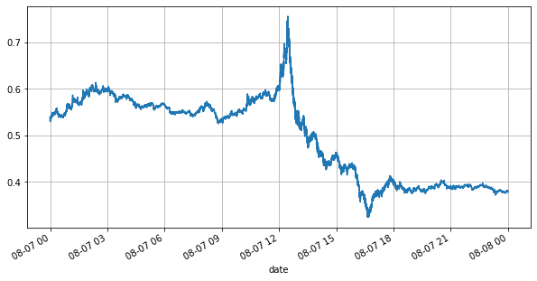
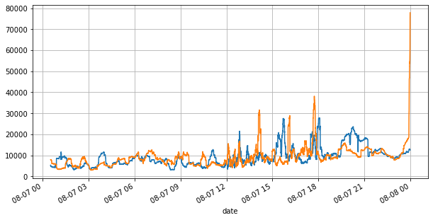
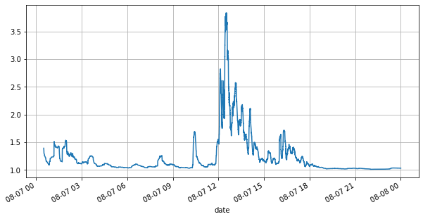
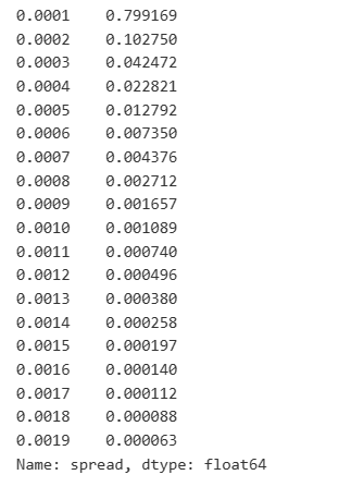
First, let's take a look at the market conditions on that day. There were large fluctuations, and the order book volume changed significantly along with the market volatility. The spread, particularly, indicated the extent of market fluctuations, which is the difference between the best ask and bid prices. In the statistics of the YGG market on that day, the spread was larger than one tick for 20% of the time. In this era of various trading bots competing in the order book, such situations are becoming increasingly rare.
In [1]:
from datetime import date,datetime
import time
import pandas as pd
import numpy as np
import matplotlib.pyplot as plt
%matplotlib inline
In [2]:
books = pd.read_csv('YGGUSDT-bookTicker-2023-08-07.csv')
In [3]:
tick_size = 0.0001
In [4]:
books['date'] = pd.to_datetime(books['transaction_time'], unit='ms')
books.index = books['date']
In [5]:
books['spread'] = round(books['best_ask_price'] - books['best_bid_price'],4)
In [6]:
books['best_bid_price'][::10].plot(figsize=(10,5),grid=True);
Out[6]:
In [7]:
books['best_bid_qty'][::10].rolling(10000).mean().plot(figsize=(10,5),grid=True);
books['best_ask_qty'][::10].rolling(10000).mean().plot(figsize=(10,5),grid=True);
Out[7]:
In [8]:
(books['spread'][::10]/tick_size).rolling(10000).mean().plot(figsize=(10,5),grid=True);
Out[8]:
In [9]:
books['spread'].value_counts()[books['spread'].value_counts()>500]/books['spread'].value_counts().sum()
Out[9]:
Imbalanced Quotes
Imbalanced quotes are observed from the significant difference in the order book volumes between the buy and sell orders most of the time. This difference has a strong predictive effect on short-term market trends, similar to the reason mentioned earlier that a decrease in buy order volume often leads to a decline. If one side of the order book is significantly smaller than the other, assuming the active buying and selling orders are similar in volume, there is a greater likelihood of the smaller side being consumed, thereby driving price changes. Imbalanced quotes are represented by the letter "I".

Where Q_b represents the amount of pending buy orders (best_bid_qty) and Q_a represents the amount of pending sell orders (best_ask_qty).
Define mid-price:

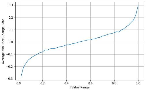
The graph below shows the relationship between the rate of change of mid-price over the next 1 interval and the imbalance I. As expected, the more likely the price is to increase as I increases and the closer it gets to 1, the more the price change accelerates. In high-frequency trading, the introduction of the intermediate price is to better predict future price changes, that is, and the future price difference is smaller, the better the intermediate price is defined. Obviously the imbalance of pending orders provides additional information for the prediction of the strategy, with this in mind, defining the weighted mid-price:

In [10]:
books['I'] = books['best_bid_qty'] / (books['best_bid_qty'] + books['best_ask_qty'])
In [11]:
books['mid_price'] = (books['best_ask_price'] + books['best_bid_price'])/2
In [12]:
bins = np.linspace(0, 1, 51)
books['I_bins'] = pd.cut(books['I'], bins, labels=bins[1:])
books['price_change'] = (books['mid_price'].pct_change()/tick_size).shift(-1)
avg_change = books.groupby('I_bins')['price_change'].mean()
plt.figure(figsize=(8,5))
plt.plot(avg_change)
plt.xlabel('I Value Range')
plt.ylabel('Average Mid Price Change Rate');
plt.grid(True)
Out[12]:
In [13]:
books['weighted_mid_price'] = books['mid_price'] + books['spread']*books['I']/2
bins = np.linspace(-1, 1, 51)
books['I_bins'] = pd.cut(books['I'], bins, labels=bins[1:])
books['weighted_price_change'] = (books['weighted_mid_price'].pct_change()/tick_size).shift(-1)
avg_change = books.groupby('I_bins')['weighted_price_change'].mean()
plt.figure(figsize=(8,5))
plt.plot(avg_change)
plt.xlabel('I Value Range')
plt.ylabel('Weighted Average Mid Price Change Rate');
plt.grid(True)
Out[13]:
Adjust Weighted Mid-Price:
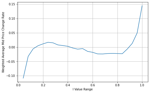
From the graph, it can be observed that the weighted mid-price shows smaller variations compared to different values of I, indicating that it is a better fit. However, there are still some deviations, particularly around 0.2 and 0.8. This suggests that I still provides additional information. The assumption of a completely linear relationship between the price correction term and I, as implied by the weighted mid-price, does not align with reality. It can be seen from the graph that the deviation speed increases when I approaches 0 and 1, indicating a non-linear relationship.
To provide a more intuitive representation, here is a redefinition of I:
Revised definition of I:

At this point:

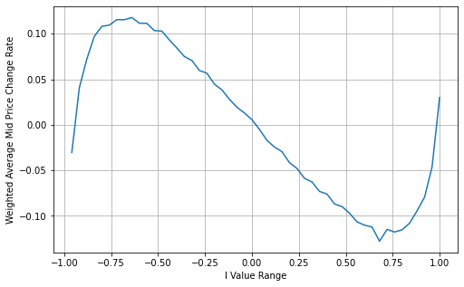
Upon observation, it can be noticed that the weighted mid-price is a correction to the average mid-price, where the correction term is multiplied by the spread. The correction term is a function of I, and the weighted mid-price assumes a simple relationship of I/2. In this case, the advantage of the adjusted I distribution (-1, 1) becomes apparent, as I is symmetric around the origin, making it convenient to find a fitting relationship for the function. By examining the graph, it appears that this function should satisfy odd powers of I, as it aligns with the rapid growth on both sides and symmetry around the origin. Additionally, it can be observed that values near the origin are close to linear. Furthermore, when I is 0, the function result is 0, and when I is 1, the function result is 0.5. Therefore, it is speculated that the function is of the form:

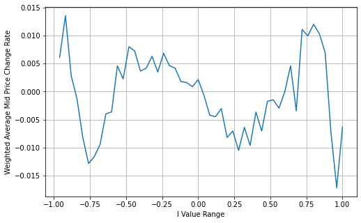
Here N is a positive even number, after actual testing, it is better when N is 8. So far this paper presents the modified weighted mid-price:

At this point, the prediction of mid-price changes is no longer significantly related to I. Although this result is slightly better than the simple weighted mid-price, it is still not applicable in real trading scenarios. This is just a proposed approach. In a 2017 article by S Stoikov, the concept of Micro-Price is introduced using a Markov chain approach, and related code is provided. Researchers can explore this approach further.
In [14]:
books['I'] = (books['best_bid_qty'] - books['best_ask_qty']) / (books['best_bid_qty'] + books['best_ask_qty'])
In [15]:
books['weighted_mid_price'] = books['mid_price'] + books['spread']*books['I']/2
bins = np.linspace(-1, 1, 51)
books['I_bins'] = pd.cut(books['I'], bins, labels=bins[1:])
books['weighted_price_change'] = (books['weighted_mid_price'].pct_change()/tick_size).shift(-1)
avg_change = books.groupby('I_bins')['weighted_price_change'].mean()
plt.figure(figsize=(8,5))
plt.plot(avg_change)
plt.xlabel('I Value Range')
plt.ylabel('Weighted Average Mid Price Change Rate');
plt.grid(True)
Out[15]:
In [16]:
books['adjust_mid_price'] = books['mid_price'] + books['spread']*books['I']*(books['I']**8+1)/4
bins = np.linspace(-1, 1, 51)
books['I_bins'] = pd.cut(books['I'], bins, labels=bins[1:])
books['adjust_mid_price'] = (books['adjust_mid_price'].pct_change()/tick_size).shift(-1)
avg_change = books.groupby('I_bins')['adjust_mid_price'].mean()
plt.figure(figsize=(8,5))
plt.plot(avg_change)
plt.xlabel('I Value Range')
plt.ylabel('Weighted Average Mid Price Change Rate');
plt.grid(True)
Out[16]:
Summary
The mid-price is crucial for high-frequency strategies as it serves as a prediction of short-term future prices. Therefore, it is important for the mid-price to be as accurate as possible. The mid-price approaches discussed earlier are based on order book data, as only the top level of the order book is utilized in the analysis. In live trading, strategies should aim to utilize all available data, including trade data, to validate mid-price predictions against actual transaction prices. I recall Stoikov mentioning in a Twitter that the real mid-price should be a weighted average of the probabilities of the bid and ask prices being executed. This issue has been explored in the previous articles. Due to length constraints, further details on these topics will be discussed in the next article.
From: https://blog.mathquant.com/2023/08/10/thoughts-on-high-frequency-trading-strategies-4.html
