Binance futures multi-currency hedging strategy's recent review and minute-level K-line backtest results
Three research reports on Binance's multi-currency hedging strategy have been published, here is the fourth one. The connection of the first three articles, you must read it again if you haven't read it, you can understand the forming idea of the strategy, the setting of specific parameters and the strategy logic.
Research on Binance Futures Multi-currency Hedging Strategy Part 1: https://www.fmz.com/digest-topic/5584
Research on Binance Futures Multi-currency Hedging Strategy Part 2: https://www.fmz.com/digest-topic/5588
Research on Binance Futures Multi-currency Hedging Strategy Part 3: https://www.fmz.com/digest-topic/5605
This article is to review the real market situation of the recent week, and summarize the gains and losses. Since crawling the Binance Futures minute K line data of the last two months, the original 1h K line backtest results can be updated, which can better explain the meaning of some parameter settings.
# Libraries to import
import pandas as pd
import requests
import matplotlib.pyplot as plt
import seaborn as sns
import numpy as np
%matplotlib inline
symbols = ['BTC','ETH', 'BCH', 'XRP', 'EOS', 'LTC', 'TRX', 'ETC', 'LINK', 'XLM', 'ADA', 'XMR', 'DASH', 'ZEC', 'XTZ', 'BNB', 'ATOM', 'ONT', 'IOTA', 'BAT', 'VET', 'NEO', 'QTUM', 'IOST']
Minutes level K line data
The data from February 21 to April 15 at two o'clock in the afternoon, a total of 77160 * 24, which greatly reduced our backtest speed, the backtest engine is not efficient enough, you can optimize it yourself. In the future, I will regularly track the latest data.
price_usdt = pd.read_csv('https://www.fmz.com/upload/asset/2b1fa7ab641385067ad.csv',index_col = 0)
price_usdt.shape
(77160, 24)
price_usdt.index = pd.to_datetime(price_usdt.index,unit='ms')
price_usdt_norm = price_usdt/price_usdt.fillna(method='bfill').iloc[0,]
price_usdt_btc = price_usdt.divide(price_usdt['BTC'],axis=0)
price_usdt_btc_norm = price_usdt_btc/price_usdt_btc.fillna(method='bfill').iloc[0,]
class Exchange:

    def __init__(self, trade_symbols, leverage=20, commission=0.00005,  initial_balance=10000, log=False):
        self.initial_balance = initial_balance # Initial asset
        self.commission = commission
        self.leverage = leverage
        self.trade_symbols = trade_symbols
        self.date = ''
        self.log = log
        self.df = pd.DataFrame(columns=['margin','total','leverage','realised_profit','unrealised_profit'])
        self.account = {'USDT':{'realised_profit':0, 'margin':0, 'unrealised_profit':0, 'total':initial_balance, 'leverage':0, 'fee':0}}
        for symbol in trade_symbols:
            self.account[symbol] = {'amount':0, 'hold_price':0, 'value':0, 'price':0, 'realised_profit':0, 'margin':0, 'unrealised_profit':0,'fee':0}

    def Trade(self, symbol, direction, price, amount, msg=''):
        if self.date and self.log:
            print('%-20s%-5s%-5s%-10.8s%-8.6s %s'%(str(self.date), symbol, 'buy' if direction == 1 else 'sell', price, amount, msg))

        cover_amount = 0 if direction*self.account[symbol]['amount'] >=0 else min(abs(self.account[symbol]['amount']), amount)
        open_amount = amount - cover_amount

        self.account['USDT']['realised_profit'] -= price*amount*self.commission # Minus handling fee
        self.account['USDT']['fee'] += price*amount*self.commission
        self.account[symbol]['fee'] += price*amount*self.commission

        if cover_amount > 0: # close position first
            self.account['USDT']['realised_profit'] += -direction*(price - self.account[symbol]['hold_price'])*cover_amount  # profit
            self.account['USDT']['margin'] -= cover_amount*self.account[symbol]['hold_price']/self.leverage # Free margin

            self.account[symbol]['realised_profit'] += -direction*(price - self.account[symbol]['hold_price'])*cover_amount
            self.account[symbol]['amount'] -= -direction*cover_amount
            self.account[symbol]['margin'] -=  cover_amount*self.account[symbol]['hold_price']/self.leverage
            self.account[symbol]['hold_price'] = 0 if self.account[symbol]['amount'] == 0 else self.account[symbol]['hold_price']

        if open_amount > 0:
            total_cost = self.account[symbol]['hold_price']*direction*self.account[symbol]['amount'] + price*open_amount
            total_amount = direction*self.account[symbol]['amount']+open_amount

            self.account['USDT']['margin'] +=  open_amount*price/self.leverage
            self.account[symbol]['hold_price'] = total_cost/total_amount
            self.account[symbol]['amount'] += direction*open_amount
            self.account[symbol]['margin'] +=  open_amount*price/self.leverage

        self.account[symbol]['unrealised_profit'] = (price - self.account[symbol]['hold_price'])*self.account[symbol]['amount']
        self.account[symbol]['price'] = price
        self.account[symbol]['value'] = abs(self.account[symbol]['amount'])*price

        return True

    def Buy(self, symbol, price, amount, msg=''):
        self.Trade(symbol, 1, price, amount, msg)

    def Sell(self, symbol, price, amount, msg=''):
        self.Trade(symbol, -1, price, amount, msg)

    def Update(self, date, close_price): # Update assets
        self.date = date
        self.close = close_price
        self.account['USDT']['unrealised_profit'] = 0
        for symbol in self.trade_symbols:
            if np.isnan(close_price[symbol]):
                continue
            self.account[symbol]['unrealised_profit'] = (close_price[symbol] - self.account[symbol]['hold_price'])*self.account[symbol]['amount']
            self.account[symbol]['price'] = close_price[symbol]
            self.account[symbol]['value'] = abs(self.account[symbol]['amount'])*close_price[symbol]
            self.account['USDT']['unrealised_profit'] += self.account[symbol]['unrealised_profit']

        self.account['USDT']['total'] = round(self.account['USDT']['realised_profit'] + self.initial_balance + self.account['USDT']['unrealised_profit'],6)
        self.account['USDT']['leverage'] = round(self.account['USDT']['margin']/self.account['USDT']['total'],4)*self.leverage
        self.df.loc[self.date] = [self.account['USDT']['margin'],self.account['USDT']['total'],self.account['USDT']['leverage'],self.account['USDT']['realised_profit'],self.account['USDT']['unrealised_profit']]
Last week review
The strategy code was released in the WeChat group on April 10th. At the beginning, a group of people ran strategy 2(short over-rise and long over-fall). In the first three days, the return was very good, and the retracement was very low. in the following days, some trader magnified the leverage, some even uses the whole amount of their funds to operate, and the gains reached 10% in one day. Strategy Square also released a lot of real market strategies, many people began to dissatisfied with the conservative recommended parameters, and have amplified the transaction volume. After April 13, due to BNB's independent trend, the profit began to retreat and sideways. If you look at the default 3% trade_value, it probably retreated 1%. However, due to the enlarged parameters values, many traders earn less and lose much. This wave of retracement was fairly timely, calming everyone down a bit.
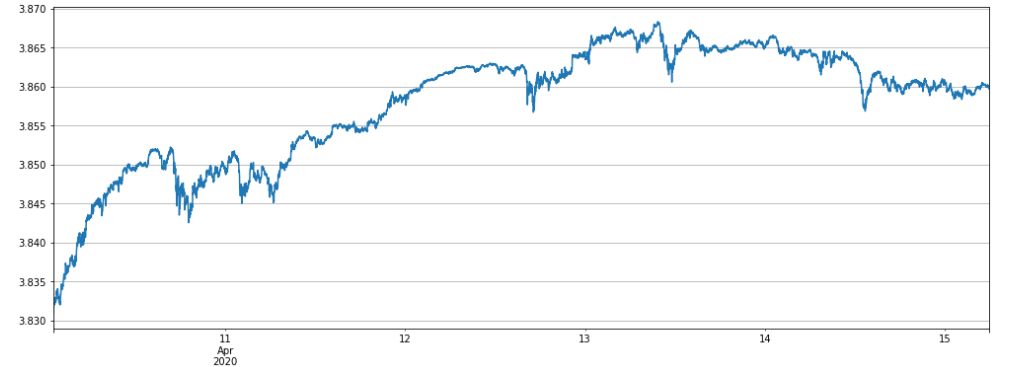
let's take a look at the full currency backtest of Strategy 2. Here, since it is a minute level update, the Alpha parameter needs to be adjusted. From a real market point of view, the curve trend is consistent, indicating that our backtest can be used as a strong reference. The net value has reached the peak of the net value from 4.13 onwards and has been in the phase of retracement and sideways.
Alpha = 0.001
#price_usdt_btc_norm2 = price_usdt_btc/price_usdt_btc.rolling(20).mean() # Ordinary moving average
price_usdt_btc_norm2 = price_usdt_btc/price_usdt_btc.ewm(alpha=Alpha).mean() # Here is consistent with the strategy, using EMA
trade_symbols = list(set(symbols))
price_usdt_btc_norm_mean = price_usdt_btc_norm2[trade_symbols].mean(axis=1)
e = Exchange(trade_symbols,initial_balance=10000,commission=0.00075,log=False)
trade_value = 300
for row in price_usdt.iloc[-7500:].iterrows():
    e.Update(row[0], row[1])
    for symbol in trade_symbols:
        price = row[1][symbol]
        if np.isnan(price):
            continue
        diff = price_usdt_btc_norm2.loc[row[0],symbol] - price_usdt_btc_norm_mean[row[0]]
        aim_value = -trade_value*round(diff/0.01,1)
        now_value = e.account[symbol]['value']*np.sign(e.account[symbol]['amount'])
        if aim_value - now_value > 0.5*trade_value:
            e.Buy(symbol, price, round((aim_value - now_value)/price, 6),round(e.account[symbol]['realised_profit']+e.account[symbol]['unrealised_profit'],2))
        if aim_value - now_value < -0.5*trade_value:
            e.Sell(symbol, price, -round((aim_value - now_value)/price, 6),round(e.account[symbol]['realised_profit']+e.account[symbol]['unrealised_profit'],2))
stragey_2a = e
(stragey_2a.df['total']/stragey_2d.initial_balance).plot(figsize=(17,6),grid = True);
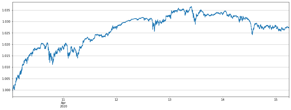
Strategy 1, short altcoin strategy achieves positive returns
trade_symbols = list(set(symbols)-set(['LINK','BTC','XTZ','BCH', 'ETH'])) # Selling short currencies
e = Exchange(trade_symbols+['BTC'],initial_balance=10000,commission=0.00075,log=False)
trade_value = 2000
for row in price_usdt.iloc[-7500:].iterrows():
    e.Update(row[0], row[1])
    empty_value = 0
    for symbol in trade_symbols:
        price = row[1][symbol]
        if np.isnan(price):
            continue
        if e.account[symbol]['value'] - trade_value  < -120 :
            e.Sell(symbol, price, round((trade_value-e.account[symbol]['value'])/price, 6),round(e.account[symbol]['realised_profit']+e.account[symbol]['unrealised_profit'],2))
        if e.account[symbol]['value'] - trade_value > 120 :
            e.Buy(symbol, price, round((e.account[symbol]['value']-trade_value)/price, 6),round(e.account[symbol]['realised_profit']+e.account[symbol]['unrealised_profit'],2))
        empty_value += e.account[symbol]['value']
    price = row[1]['BTC']
    if e.account['BTC']['value'] - empty_value < -120:
        e.Buy('BTC', price, round((empty_value-e.account['BTC']['value'])/price,6),round(e.account['BTC']['realised_profit']+e.account['BTC']['unrealised_profit'],2))
    if e.account['BTC']['value'] - empty_value > 120:
        e.Sell('BTC', price, round((e.account['BTC']['value']-empty_value)/price,6),round(e.account['BTC']['realised_profit']+e.account['BTC']['unrealised_profit'],2))
stragey_1 = e
(stragey_1.df['total']/stragey_1.initial_balance).plot(figsize=(17,6),grid = True);
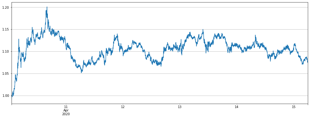
Strategy 2 buying Long over-fall and selling short over-rise profit analysis
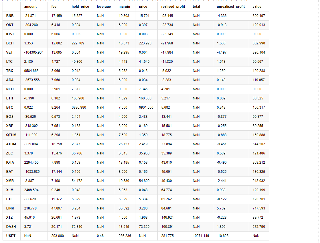
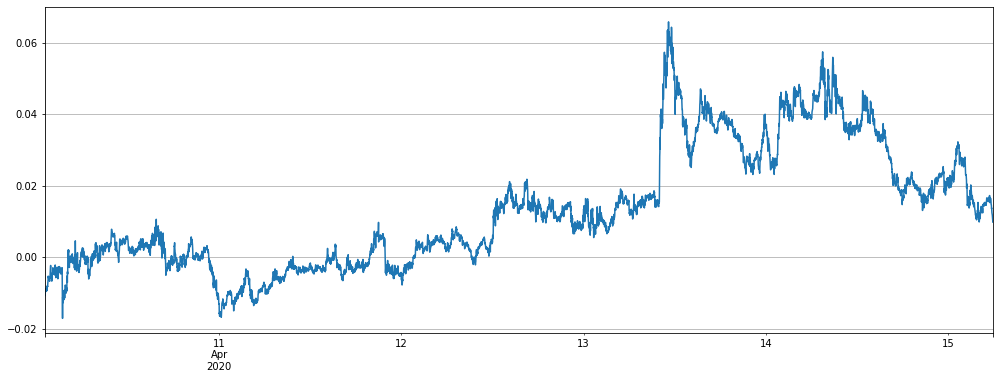
Printing out the final account information shows that most currencies have brought profits, and BNB has suffered the most losses. This is also mainly because BNB has gone out of a wave of independent trend, rising a lot, and the largest deviation is 0.06.
pd.DataFrame(stragey_2a.account).T.apply(lambda x:round(x,3)).sort_values(by='realised_profit')
# BNB deviation
(price_usdt_btc_norm2.iloc[-7500:].BNB-price_usdt_btc_norm_mean[-7500:]).plot(figsize=(17,6),grid = True);
#price_usdt_btc_norm_mean[-7500:].plot(figsize=(17,6),grid = True);
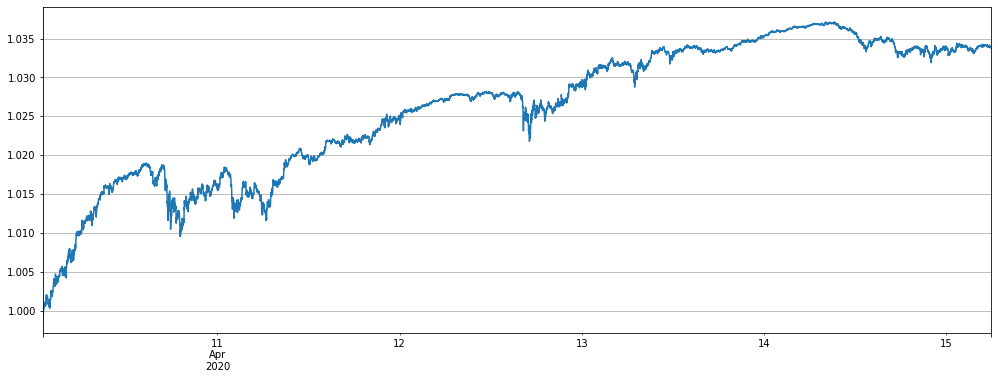
If BNB and ATOM are removed, the result is better, but the strategy will still be in the retracement stage recently.
Alpha = 0.001
price_usdt_btc_norm2 = price_usdt_btc/price_usdt_btc.ewm(alpha=Alpha).mean() # Here is consistent with the strategy, using EMA
trade_symbols = list(set(symbols)-set(['BNB','ATOM']))
price_usdt_btc_norm_mean = price_usdt_btc_norm2[trade_symbols].mean(axis=1)
e = Exchange(trade_symbols,initial_balance=10000,commission=0.00075,log=False)
trade_value = 300
for row in price_usdt.iloc[-7500:].iterrows():
    e.Update(row[0], row[1])
    for symbol in trade_symbols:
        price = row[1][symbol]
        if np.isnan(price):
            continue
        diff = price_usdt_btc_norm2.loc[row[0],symbol] - price_usdt_btc_norm_mean[row[0]]
        aim_value = -trade_value*round(diff/0.01,1)
        now_value = e.account[symbol]['value']*np.sign(e.account[symbol]['amount'])
        if aim_value - now_value > 0.5*trade_value:
            e.Buy(symbol, price, round((aim_value - now_value)/price, 6),round(e.account[symbol]['realised_profit']+e.account[symbol]['unrealised_profit'],2))
        if aim_value - now_value < -0.5*trade_value:
            e.Sell(symbol, price, -round((aim_value - now_value)/price, 6),round(e.account[symbol]['realised_profit']+e.account[symbol]['unrealised_profit'],2))
stragey_2b = e
(stragey_2b.df['total']/stragey_2b.initial_balance).plot(figsize=(17,6),grid = True);
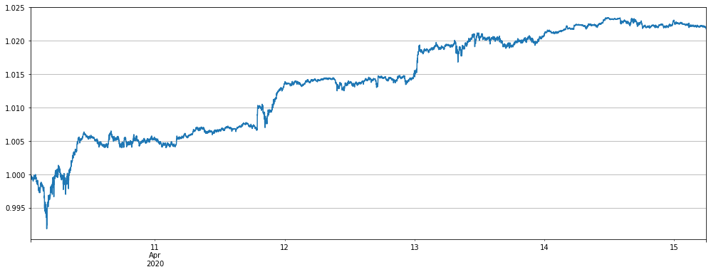
In the past two days, it has become popular to run mainstream currency strategies. Let's backtest this strategy. Due to the decrease in currency variety, trade_value was appropriately increased by 4 times for comparison, and the results performed well, especially since the recent retracement was small.
It should be noted that only the mainstream currency is not as good as the full currency in the longer time backtest, and there are more retracements. You can do your own backtest on the hourly line below, mainly because the currency is less dispersed and the volatility rises instead.
Alpha = 0.001
price_usdt_btc_norm2 = price_usdt_btc/price_usdt_btc.ewm(alpha=Alpha).mean() # Here is consistent with the strategy, using EMA
trade_symbols = ['ETH','LTC','EOS','XRP','BCH']
price_usdt_btc_norm_mean = price_usdt_btc_norm2[trade_symbols].mean(axis=1)
e = Exchange(trade_symbols,initial_balance=10000,commission=0.00075,log=False)
trade_value = 1200
for row in price_usdt.iloc[-7500:].iterrows():
    e.Update(row[0], row[1])
    for symbol in trade_symbols:
        price = row[1][symbol]
        if np.isnan(price):
            continue
        diff = price_usdt_btc_norm2.loc[row[0],symbol] - price_usdt_btc_norm_mean[row[0]]
        aim_value = -trade_value*round(diff/0.01,1)
        now_value = e.account[symbol]['value']*np.sign(e.account[symbol]['amount'])
        if aim_value - now_value > 0.5*trade_value:
            e.Buy(symbol, price, round((aim_value - now_value)/price, 6),round(e.account[symbol]['realised_profit']+e.account[symbol]['unrealised_profit'],2))
        if aim_value - now_value < -0.5*trade_value:
            e.Sell(symbol, price, -round((aim_value - now_value)/price, 6),round(e.account[symbol]['realised_profit']+e.account[symbol]['unrealised_profit'],2))
stragey_2c = e
(stragey_2c.df['total']/e.initial_balance).plot(figsize=(17,6),grid = True);
Handling fee and strategy parameter analysis
Since the first few reports used the hour level k line, and the actual parameters are very different with the real market situations, now with the minutes level k line, you can see how to set some parameters. First look at the default parameter settings:
Alpha = 0.03 The Alpha parameter of the exponential moving average. The larger the setting, the more sensitive the benchmark price tracking and the fewer transactions. The final holding position will also be lower, which reduces the leverage, but also will reduce the return and the maximum retracements.
Update_base_price_time_interval = 30 * 60 How often to update the base price, in seconds, related to the Alpha parameter, the smaller the Alpha setting, the smaller the interval can be set
Trade_value: Every 1% of the altcoin price (BTC-denominated) deviates from the index holding value, which needs to be determined according to the total funds invested and risk preference. It is recommended to set 3-10% of the total funds. You can look at the size of the lever through the backtest of the research environment. Trade_value can be less than Adjust_value, such as half of Adjust_value, which is equivalent to the holding value of 2% from the index.
Adjust_value: The contract value (USDT valuation) adjusts the deviation value. When the index deviates from * Trade_value-current position> Adjust_value, that is, the difference between the target position and the current position exceeds this value, trading will start. Too large adjustments are slow, too small transactions are frequent and cannot be less than 10, otherwise the minimum transaction will not be reached, it is recommended to set it to more than 40% of Trade_value.
Needless to say, Trade_value is directly related to our earnings and risks. If Trade_value has not been changed, it should be profitable so far.
Since Alpha has higher frequency data this time, it is obviously more reasonable to update it every 1 minute. Naturally, it is smaller than the original one. The specific number can be determined by backtest.
Adjust_value has always recommended more than 40% of Trade_value. The original 1h K line setting has little effect. Some people want to adjust it very low, so that it can be closer to the target position. Here we will analyze why it should not be done.
First analyze the problem of handling fees
It can be seen that under the default rate of 0.00075, the handling fee is 293 and the profit is 270, which is a very high proportion. We set the handling fee to 0 and Adjust_value to 10 to see what happens.
stragey_2a.account['USDT']
{'fee': 293.85972778530453,
 'leverage': 0.45999999999999996,
 'margin': 236.23559736312995,
 'realised_profit': 281.77464608744435,
 'total': 10271.146238,
 'unrealised_profit': -10.628408369648495}
Alpha = 0.001
#price_usdt_btc_norm2 = price_usdt_btc/price_usdt_btc.rolling(20).mean() # Ordinary moving average
price_usdt_btc_norm2 = price_usdt_btc/price_usdt_btc.ewm(alpha=Alpha).mean() # Here is consistent with the strategy, using EMA
trade_symbols = list(set(symbols))
price_usdt_btc_norm_mean = price_usdt_btc_norm2[trade_symbols].mean(axis=1)
e = Exchange(trade_symbols,initial_balance=10000,commission=0,log=False)
trade_value = 300
for row in price_usdt.iloc[-7500:].iterrows():
    e.Update(row[0], row[1])
    for symbol in trade_symbols:
        price = row[1][symbol]
        if np.isnan(price):
            continue
        diff = price_usdt_btc_norm2.loc[row[0],symbol] - price_usdt_btc_norm_mean[row[0]]
        aim_value = -trade_value*round(diff/0.01,1)
        now_value = e.account[symbol]['value']*np.sign(e.account[symbol]['amount'])
        if aim_value - now_value > 10:
            e.Buy(symbol, price, round((aim_value - now_value)/price, 6),round(e.account[symbol]['realised_profit']+e.account[symbol]['unrealised_profit'],2))
        if aim_value - now_value < 10:
            e.Sell(symbol, price, -round((aim_value - now_value)/price, 6),round(e.account[symbol]['realised_profit']+e.account[symbol]['unrealised_profit'],2))
stragey_2d = e
(stragey_2d.df['total']/e.initial_balance).plot(figsize=(17,6),grid = True);
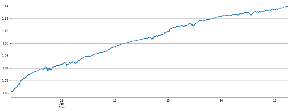
The result is a straight line upwards, BNB only brings a little twists and turns, the lower Adjust_value catches every fluctuation. If there is no handling fees, the profit will be excellent.
What if the adjustment_value is small if there is a small amount of handling fee?
Alpha = 0.001
#price_usdt_btc_norm2 = price_usdt_btc/price_usdt_btc.rolling(20).mean() # Ordinary moving average
price_usdt_btc_norm2 = price_usdt_btc/price_usdt_btc.ewm(alpha=Alpha).mean() # Here is consistent with the strategy, using EMA
trade_symbols = list(set(symbols))
price_usdt_btc_norm_mean = price_usdt_btc_norm2[trade_symbols].mean(axis=1)
e = Exchange(trade_symbols,initial_balance=10000,commission=0.00075,log=False)
trade_value = 300
for row in price_usdt.iloc[-7500:].iterrows():
    e.Update(row[0], row[1])
    for symbol in trade_symbols:
        price = row[1][symbol]
        if np.isnan(price):
            continue
        diff = price_usdt_btc_norm2.loc[row[0],symbol] - price_usdt_btc_norm_mean[row[0]]
        aim_value = -trade_value*round(diff/0.01,1)
        now_value = e.account[symbol]['value']*np.sign(e.account[symbol]['amount'])
        if aim_value - now_value > 10:
            e.Buy(symbol, price, round((aim_value - now_value)/price, 6),round(e.account[symbol]['realised_profit']+e.account[symbol]['unrealised_profit'],2))
        if aim_value - now_value < 10:
            e.Sell(symbol, price, -round((aim_value - now_value)/price, 6),round(e.account[symbol]['realised_profit']+e.account[symbol]['unrealised_profit'],2))
stragey_2e = e
(stragey_2e.df['total']/e.initial_balance).plot(figsize=(17,6),grid = True);
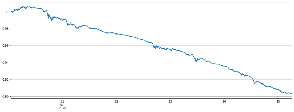
As a result, it also came out of a straight-line downward curve. It's easy to understand if you think about it, frequent adjustments within a small spread will only lose the handling fee.
Taken together, the lower the fee level, the smaller the Adjust_value can be set, the more frequent the transaction, and the higher the profit.
Problems with Alpha settings
Since there is a minute line, the benchmark price will be updated once a minute, here we simply backtest to determine the size of alpha. The current recommended Alpha setting is 0.001.
for Alpha in [0.0001, 0.0003, 0.0006, 0.001, 0.0015, 0.002, 0.004, 0.01, 0.02]:
#price_usdt_btc_norm2 = price_usdt_btc/price_usdt_btc.rolling(20).mean() # Ordinary moving average
    price_usdt_btc_norm2 = price_usdt_btc/price_usdt_btc.ewm(alpha=Alpha).mean() #Here is consistent with the strategy, using EMA
    trade_symbols = list(set(symbols))
    price_usdt_btc_norm_mean = price_usdt_btc_norm2[trade_symbols].mean(axis=1)
    e = Exchange(trade_symbols,initial_balance=10000,commission=0.00075,log=False)
    trade_value = 300
    for row in price_usdt.iloc[-7500:].iterrows():
        e.Update(row[0], row[1])
        for symbol in trade_symbols:
            price = row[1][symbol]
            if np.isnan(price):
                continue
            diff = price_usdt_btc_norm2.loc[row[0],symbol] - price_usdt_btc_norm_mean[row[0]]
            aim_value = -trade_value*round(diff/0.01,1)
            now_value = e.account[symbol]['value']*np.sign(e.account[symbol]['amount'])
            if aim_value - now_value > 0.5*trade_value:
                e.Buy(symbol, price, round((aim_value - now_value)/price, 6),round(e.account[symbol]['realised_profit']+e.account[symbol]['unrealised_profit'],2))
            if aim_value - now_value < -0.5*trade_value:
                e.Sell(symbol, price, -round((aim_value - now_value)/price, 6),round(e.account[symbol]['realised_profit']+e.account[symbol]['unrealised_profit'],2))
    print(Alpha, e.account['USDT']['unrealised_profit']+e.account['USDT']['realised_profit'])
0.0001 -77.80281760941007
0.0003 179.38803796199724
0.0006 218.12579924541367
0.001 271.1462377177959
0.0015 250.0014065973528
0.002 207.38692166891275
0.004 129.08021828803027
0.01 65.12410041648158
0.02 58.62356792410955
Backtest results of the minute line in the last two months
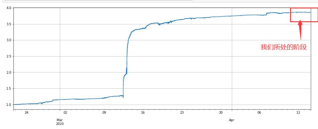
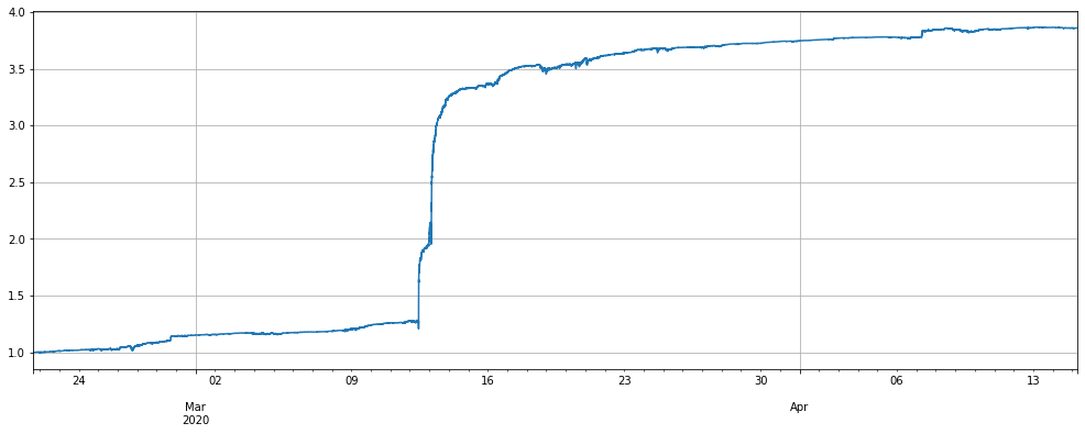
Finally, look at the results of a long time backtest. Just now, one after another rise, and today's net worth is at a new low. Let's give you the following confidence. Because the frequency of the minute line is higher, it will open and close positions within the hour, so the profit will be much higher.
Another point, we have always been using a fixed trade_value, which makes the utilization of funds in the later period insufficient, and the actual rate of return can still increase a lot.
Where are we in the two-month backtest period?
Alpha = 0.001
#price_usdt_btc_norm2 = price_usdt_btc/price_usdt_btc.rolling(20).mean() # Ordinary moving average
price_usdt_btc_norm2 = price_usdt_btc/price_usdt_btc.ewm(alpha=Alpha).mean() # Here is consistent with the strategy, using EMA
trade_symbols = list(set(symbols))
price_usdt_btc_norm_mean = price_usdt_btc_norm2[trade_symbols].mean(axis=1)
e = Exchange(trade_symbols,initial_balance=10000,commission=0.00075,log=False)
trade_value = 300
for row in price_usdt.iloc[:].iterrows():
    e.Update(row[0], row[1])
    for symbol in trade_symbols:
        price = row[1][symbol]
        if np.isnan(price):
            continue
        diff = price_usdt_btc_norm2.loc[row[0],symbol] - price_usdt_btc_norm_mean[row[0]]
        aim_value = -trade_value*round(diff/0.01,1)
        now_value = e.account[symbol]['value']*np.sign(e.account[symbol]['amount'])
        if aim_value - now_value > 0.5*trade_value:
            e.Buy(symbol, price, round((aim_value - now_value)/price, 6),round(e.account[symbol]['realised_profit']+e.account[symbol]['unrealised_profit'],2))
        if aim_value - now_value < -0.5*trade_value:
            e.Sell(symbol, price, -round((aim_value - now_value)/price, 6),round(e.account[symbol]['realised_profit']+e.account[symbol]['unrealised_profit'],2))
stragey_2f = e
(stragey_2f.df['total']/stragey_2e.initial_balance).plot(figsize=(17,6),grid = True);
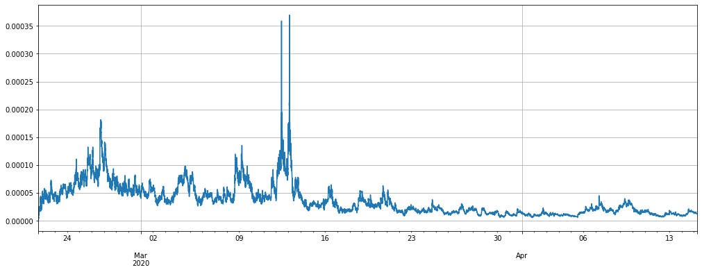
(stragey_2f.df['leverage']/stragey_2e.initial_balance).plot(figsize=(17,6),grid = True);
