The perpetual grid strategy is a popular classic strategy on FMZ platform. Compared with the spot grid, there is no need to have currencies, and leverage can be added, which is much more convenient than the spot grid. However, since it is not possible to backtest on the FMZ Quant Platform directly, it is not conducive to screening currencies and determining parameter optimization. In this article, we will introduce the complete Python backtesting process, including data collection, backtesting framework, backtesting functions, parameter optimization, etc. You can try it yourself in juypter notebook.
Data Collection
Generally, it is enough to use K-line data. For accuracy, the smaller the K-line period, the better. However, to balance the backtest time and data volume, in this article, we use 5min of data from the past two years for backtesting. The final data volume exceeded 200,000 lines. We choose DYDX as the currency. Of course, the specific currency and K-line period can be selected according to your own interests.
import requests
from datetime import date,datetime
import time
import pandas as pd
import numpy as np
import matplotlib.pyplot as plt
import requests, zipfile, io
%matplotlib inline

def GetKlines(symbol='BTC',start='2020-8-10',end='2021-8-10',period='1h'):
    Klines = []
    start_time = int(time.mktime(datetime.strptime(start, "%Y-%m-%d").timetuple()))*1000
    end_time = int(time.mktime(datetime.strptime(end, "%Y-%m-%d").timetuple()))*1000
    while start_time < end_time:
        res = requests.get('https://fapi.binance.com/fapi/v1/klines?symbol=%sUSDT&interval=%s&startTime=%s&limit=1000'%(symbol,period,start_time))
        res_list = res.json()
        Klines += res_list
        start_time = res_list[-1][0]
    return pd.DataFrame(Klines,columns=['time','open','high','low','close','amount','end_time','volume','count','buy_amount','buy_volume','null']).astype('float')

df = GetKlines(symbol='DYDX',start='2022-1-1',end='2023-12-7',period='5m')
df = df.drop_duplicates()
Backtesting Framework
For backtesting, we continue to choose the commonly used framework that supports USDT perpetual contracts in multiple currencies, which is simple and easy to use.
class Exchange:

    def __init__(self, trade_symbols, fee=0.0004, initial_balance=10000):
        self.initial_balance = initial_balance #Initial assets
        self.fee = fee
        self.trade_symbols = trade_symbols
        self.account = {'USDT':{'realised_profit':0, 'unrealised_profit':0, 'total':initial_balance, 'fee':0}}
        for symbol in trade_symbols:
            self.account[symbol] = {'amount':0, 'hold_price':0, 'value':0, 'price':0, 'realised_profit':0,'unrealised_profit':0,'fee':0}

    def Trade(self, symbol, direction, price, amount):

        cover_amount = 0 if direction*self.account[symbol]['amount'] >=0 else min(abs(self.account[symbol]['amount']), amount)
        open_amount = amount - cover_amount
        self.account['USDT']['realised_profit'] -= price*amount*self.fee #Deduction of handling fee
        self.account['USDT']['fee'] += price*amount*self.fee
        self.account[symbol]['fee'] += price*amount*self.fee

        if cover_amount > 0: #Close the position first.
            self.account['USDT']['realised_profit'] += -direction*(price - self.account[symbol]['hold_price'])*cover_amount  #Profits
            self.account[symbol]['realised_profit'] += -direction*(price - self.account[symbol]['hold_price'])*cover_amount

            self.account[symbol]['amount'] -= -direction*cover_amount
            self.account[symbol]['hold_price'] = 0 if self.account[symbol]['amount'] == 0 else self.account[symbol]['hold_price']

        if open_amount > 0:
            total_cost = self.account[symbol]['hold_price']*direction*self.account[symbol]['amount'] + price*open_amount
            total_amount = direction*self.account[symbol]['amount']+open_amount

            self.account[symbol]['hold_price'] = total_cost/total_amount
            self.account[symbol]['amount'] += direction*open_amount


    def Buy(self, symbol, price, amount):
        self.Trade(symbol, 1, price, amount)

    def Sell(self, symbol, price, amount):
        self.Trade(symbol, -1, price, amount)

    def Update(self, close_price): #Updating of assets
        self.account['USDT']['unrealised_profit'] = 0
        for symbol in self.trade_symbols:
            self.account[symbol]['unrealised_profit'] = (close_price[symbol] - self.account[symbol]['hold_price'])*self.account[symbol]['amount']
            self.account[symbol]['price'] = close_price[symbol]
            self.account[symbol]['value'] = abs(self.account[symbol]['amount'])*close_price[symbol]
            self.account['USDT']['unrealised_profit'] += self.account[symbol]['unrealised_profit']
        self.account['USDT']['total'] = round(self.account['USDT']['realised_profit'] + self.initial_balance + self.account['USDT']['unrealised_profit'],6)
Grid Backtest Function
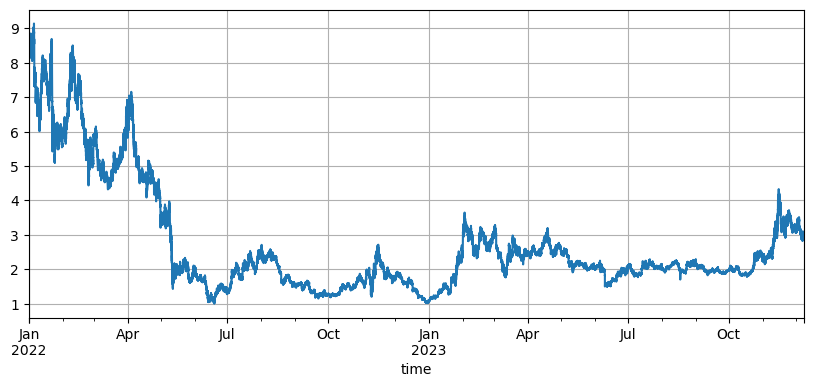
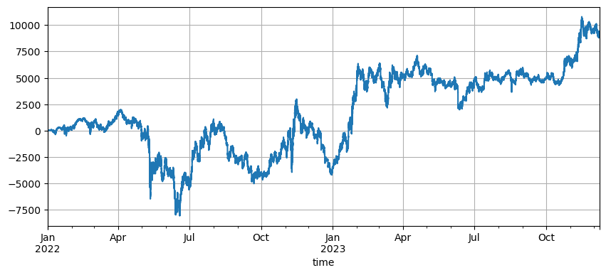
The principle of the grid strategy is very simple. Sell when the price rises and buy when the price falls. It specifically involves three parameters: initial price, grid spacing, and trading value. The market of DYDX fluctuates greatly. It fell from the initial low of 8.6U to 1U, and then rose back to 3U in the recent bull market. The default initial price of the strategy is 8.6U, which is very unfavorable for the grid strategy, but the default parameters backtested a total profit of 9200U was made in two years, and a loss of 7500U was made during the period.

symbol = 'DYDX'
value = 100
pct = 0.01

def Grid(fee=0.0002, value=100, pct=0.01, init = df.close[0]):
    e = Exchange([symbol], fee=0.0002, initial_balance=10000)
    init_price = init
    res_list = [] #For storing intermediate results
    for row in df.iterrows():
        kline = row[1] #To backtest a K-line will only generate one buy order or one sell order, which is not particularly accurate.
        buy_price = (value / pct - value) / ((value / pct) / init_price + e.account[symbol]['amount']) #The buy order price, as it is a pending order transaction, is also the final aggregated price
        sell_price = (value / pct + value) / ((value / pct) / init_price + e.account[symbol]['amount'])
        if kline.low < buy_price: #The lowest price of the K-line is lower than the current pending order price, the buy order is filled
            e.Buy(symbol,buy_price,value/buy_price)
        if kline.high > sell_price:
            e.Sell(symbol,sell_price,value/sell_price)
        e.Update({symbol:kline.close})
        res_list.append([kline.time, kline.close, e.account[symbol]['amount'], e.account['USDT']['total']-e.initial_balance,e.account['USDT']['fee'] ])
    res = pd.DataFrame(data=res_list, columns=['time','price','amount','profit', 'fee'])
    res.index = pd.to_datetime(res.time,unit='ms')
    return res

Initial Price Impact
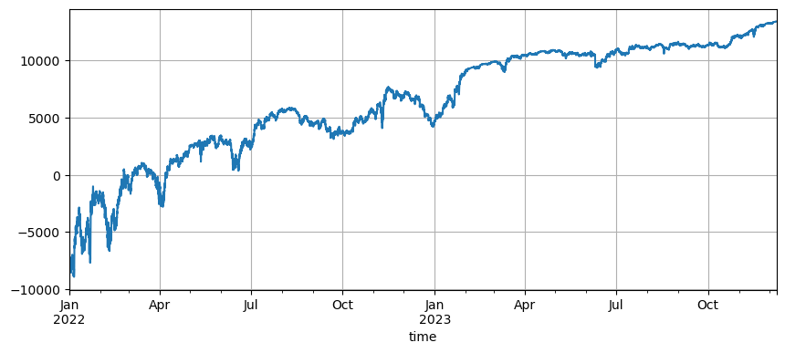
The setting of the initial price affects the initial position of the strategy. The default initial price for the backtest just now is the initial price at startup, that is, no position is held at startup. And we know that the grid strategy will realize all profits when the price returns to the initial stage, so if the strategy can correctly predict the future market when it is launched, the income will be significantly improved. Here, we set the initial price to 3U and then backtest. In the end, the maximum drawdown was 9200U, and the final profit was 13372U. The final strategy does not hold positions. The profit is all the fluctuation profits, and the difference between the profits of the default parameters is the position loss caused by inaccurate judgment of the final price.
However, if the initial price is set to 3U, the strategy will go short at the beginning and hold a large number of short positions. In this example, a short order of 17,000 U is directly held, so it faces greater risks.

Grid Spacing Settings
The grid spacing determines the distance between pending orders. Obviously, the smaller the spacing, the more frequent the transactions, the lower the profit of a single transaction, and the higher the handling fee. However, it is worth noting that as the grid spacing becomes smaller and the grid value remains unchanged, when the price changes, the total positions will increase, and the risks faced are completely different. Therefore, to backtest the effect of grid spacing, it is necessary to convert the grid value.
Since the backtest uses 5m K-line data, and each K-line is only traded once, which is obviously unrealistic, especially since the volatility of digital currencies is very high. A smaller spacing will miss many transactions in backtesting compared with the live trading. Only a larger spacing will have reference value. In this backtesting mechanism, the conclusions drawn are not accurate. Through tick-level order flow data backtesting, the optimal grid spacing should be 0.005-0.01.
for p in [0.0005, 0.001 ,0.002 ,0.005, 0.01, 0.02, 0.05]:
    res = Grid( fee=0.0002, value=value*p/0.01, pct=p, init =3)
    print(p, round(min(res['profit']),0), round(res['profit'][-1],0), round(res['fee'][-1],0))

0.0005 -8378.0 144.0 237.0
0.001 -9323.0 1031.0 465.0
0.002 -9306.0 3606.0 738.0
0.005 -9267.0 9457.0 781.0
0.01 -9228.0 13375.0 550.0
0.02 -9183.0 15212.0 309.0
0.05 -9037.0 16263.0 131.0
Grid Transaction Value
As mentioned before, when the fluctuations are the same, the greater the value of the holding, the risk is proportional. However, as long as there is no rapid decline, 1% of the total funds and 1% of the grid spacing should be able to cope with most market conditions. In this DYDX example, a drop of almost 90% also triggered a liquidation. However, it should be noted that DYDX mainly falls. When the grid strategy goes long when it falls, it will fall by 100% at most, while there is no limit on the rise, and the risk is much higher. Therefore, Grid Strategy recommends users to choose only the long position mode for currencies they believe have potential.
