High-frequency backtest system based on each transaction and the defects of K-line backtest
When I wrote Research on Binance Futures Multi-currency Hedging Strategy, I also released a backtest engine. And the first report was based on the one-hour K-line backtest, which verified the effectiveness of the strategy. But the sleep time of the actual open sourced strategy is "1 second", which is a fairly high-frequency strategy. Obviously, using the hourly K-line backtest cannot produce accurate results. Later on, the results of the backtest of the minute level K line were added, and the backtest revenue has improved a lot, but it is still impossible to determine what parameters should be used in the case of "seconds level", and the understanding of the entire strategy is not very clear. The main reason is the important drawback of backtest based on K-line.
Problems based on K-line backtest
First of all, what is the historical K line? A K-line data contains four prices of high, open, low, close, the first two "times" and the volume of the interval. Most quantization platforms and frameworks are based on K-line backtest, and the FMZ platform also provides tick-level backtest. K line backtest speed is very fast, and in most cases it has very few issues, but it also has very serious defects, especially the backtest multi-variety strategy and high-frequency strategy, it is almost impossible to draw a correct conclusion.
The first is the issue of time. The time of the highest price and the lowest price of the K-line data is not given and need not be considered, but the most important opening and closing prices are not the opening and closing time. Even the less popular trading varieties often have no trade for more than ten seconds, and when we backtest the multi-variety strategy, we often assume that their opening price and closing price are the same, which is also based on the backtest of the closing price.
Imagine using the minute level K line to backtest the arbitrage of two varieties. The difference between them is usually 10 yuan(or dollars). Now, at 10:01, the closing price of contract A is 100, the contract B is 112, and the difference is 12 yuan. So the strategy begins to hedge. At certain moment, the price difference returned, and the strategy made a return profit of 2 yuan.
but the actual situation may be that at 10:00:45, contract A produced a transaction of 100 yuan, after which there was no transaction, contract B had a transaction of 112 yuan at 10:00:58, at 10:01:00 Both prices do not exist. What is the market price at this time, and how much can the hedge operation get? I can’t know. One possible situation is: at 10:00:58, the "Buy 1" and "Sell 1" pending order price of contract A is 101.9 to 102.1, and there is no difference of 2 yuan at all. This will greatly mislead our strategy optimization.
The second is the matchmaking problem. The real matchmaking is price priority and time priority. If the buyer exceeds the "Sell 1" price, they will usually directly deal at the "Sell 1" price, otherwise they will enter the pending order book and wait. The K line data obviously does not have "Buy 1" and "Sell 1" price, it is impossible to simulate the level of detail price matching.
The last is the impact of the strategy itself on the market. If it is a backtest of small amount funds, the impact is not large. But if the volume of transactions is large, it will have an impact on the market. Not only will the price slippage be large when you placing a large volume order, if you buying long order executed, this kind of action actually seize the orders of other traders who originally wanted to buy, the "butterfly" effect will have an impact on the market. This effect cannot be quantified. We can only tell from experience that high-frequency trading can only accommodate small funds.
Backtest based on real-time depth and tick
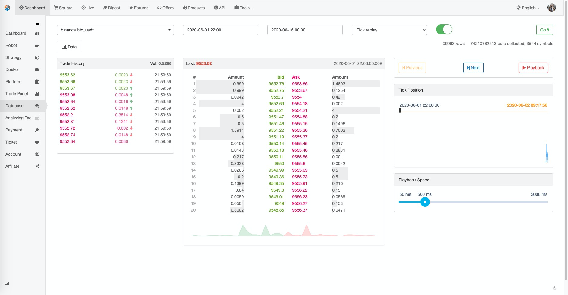
FMZ provides real-level backtest, which can obtain real historical 20 layer depth price, real-time second-level Ticks, Each Individual Transaction and other data. Based on these features, FMZ made a real-time transaction playback function.
This kind of amount of backtest data is very large, and the backtest speed is also very slow, generally only can backtest for two days. For relatively high-frequency or time-critical strategies, real market level backtest is necessary. The trading pairs and trading time collected by FMZ are not very long, but there are still more than 70 billion historical data.
The current matchmaking mechanism is that if the buying order is greater than the "Sell 1", it will be completely matched immediately without looking at the amount, and if it is less than the "Sell 1", it will enter the match queue to wait. Such backtest mechanism solves the first two problems of K-line backtest, but still cannot solve the last problem. And because the amount of data is too large, the backtest speed and time range are limited.

Backtest mechanism based on order-by-order transaction flow
There is too little information in the K line, and the price depth may also be a fake depth, but there is a kind of data that is the market's real transaction willingness, which reflects the most real transaction history, that is, Each Individual Transaction. This article will propose a high-frequency backtest system based on the order flow, which will greatly reduce the volume of real market level backtest data, and to a certain extent simulate the impact of trading volume on the market.
I downloaded the transaction of the last 5 days Binance XTZ perpetual contract (download address: https://www.fmz.com/upload/asset/1ff487b007e1a848ead.csv), as a not popular variety, it has a total of 213000 transaction data, first let's look at the composition of the data:
[['XTZ', 1590981301905, 2.905, 0.4, 'False\n'],
 ['XTZ', 1590981303044, 2.903, 3.6, 'True\n'],
 ['XTZ', 1590981303309, 2.903, 3.7, 'True\n'],
 ['XTZ', 1590981303738, 2.903, 238.1, 'True\n'],
 ['XTZ', 1590981303892, 2.904, 0.1, 'False\n'],
 ['XTZ', 1590981305250, 2.904, 0.1, 'False\n'],
 ['XTZ', 1590981305643, 2.903, 197.3, 'True\n'],
The data is a two-dimensional list, sorted in chronological order. The specific meanings are as follows: variety name, transaction price, transaction timestamp, transaction quantity, whether it is a selling order active transaction. There are buying and selling side, and each transaction includes the buyer and the seller. If the buyer is a market Maker and the seller is an active Taker, the last data is True.
First of all, according to the direction of the transaction, you can quite accurately speculate on the "Buy 1" and "Sell 1" in the market. If it is an active selling order, then the "Buy 1" price at this time is the transaction price, if it is an active buying order, the "Sell 1" price will be the transaction price. If there is a new transaction, then all the price will be renewed and updated. The last result will be retained if there is no renew and update. It is easy to introduce the last moment of the above data, the "Buy 1" price is 2.903, and the "Sell 1" is 2.904.
According to the order flow, it can be matched in this way: take a buying order as an example, the price is price, the order quantity is amount, then buy and sell 1 at this time are bid and ask respectively. If price is lower than ask and higher than bid, then it is judged as maker first, and priority can be matched to make a deal, then all the deals with a transaction price lower than or equal the price during the order existence time will be matched with this order (if price is lower or equal to bid, no priority is given to the transaction. Orders with a transaction price lower than price are matched with this order.)
The matching price is price, and the volume is the transaction volume of Each Individual Transaction, until the order is fully completed or the order is cancelled. If the price is higher than ask, it is judged as a taker. After that, during the time when the order exists, all the deals with a transaction price lower than or equal to price are matched with this order, and the match price is the transaction price of the Each Individual Transaction. The distinction between maker and taker are basically because the exchange encourages pending orders and there are discounts for transaction fees. For high-frequency strategies, this difference must be considered.
It is easy to see a problem with this kind of matching. If the order is a taker, the actual situation is that it can be executed immediately, rather than waiting for a new order to be matched with it. First of all, we did not consider the volume of pending orders, even if there are some data, directly judge the transaction has also changed the price depth, affecting the market.
Based on the matching of new orders, it is equivalent to replacing the existing orders in history with your orders. In any case, it will not exceed the limit of the market's own trading volume, and the ultimate profit cannot exceed the maximum profit generated by the market. Part of the matching mechanism also affects the volume of orders, which in turn affects the strategy's revenue, quantitatively reflecting the strategy's capacity. There will be no traditional backtest, when the amount of funds doubles and the gain doubles.
There are still some small details. If the buying price of the order is equal to "Buy 1", there is still a certain probability that the buying price will be matched by "Buy 1", this kind of situation will not be considered here.
Matching code
Exchange objects can refer to the introduction at the beginning, basically unchanged, only adding the difference between maker and taker fees, and optimizing the speed of backtest. The following will mainly introduce the matching code.
 symbol = 'XTZ'
    loop_time = 0
    intervel = 1000 # The sleep time of the strategy is 1000ms
    init_price = data[0][2] # Initial price
    e = Exchange([symbol],initial_balance=1000000,maker_fee=maker_fee,taker_fee=taker_fee,log='') # Initialize the exchange
    depth = {'ask':data[0][2], 'bid':data[0][2]} # depth
    order = {'buy':{'price':0,'amount':0,'maker':False,'priority':False,'id':0},
             'sell':{'price':0,'amount':0,'maker':False,'priority':False,'id':0}} # order
    for tick in data:
        price = int(tick[2]/tick_sizes[symbol])*tick_sizes[symbol] # executed price
        trade_amount = tick[3] # executed volume
        time_stamp = tick[1] # executed timestamp
        if tick[4] == 'False\n':
            depth['ask'] = price
        else:
            depth['bid'] = price

        if depth['bid'] < order['buy']['price']:
            order['buy']['priority'] = True
        if depth['ask'] > order['sell']['price']:
            order['sell']['priority'] = True
        if price > order['buy']['price']:
            order['buy']['maker'] = True
        if price < order['sell']['price']:
            order['sell']['maker'] = True

        # Order network delay can also be used as one of the matching conditions, not considered here
        cond1 = order['buy']['priority'] and order['buy']['price'] >= price and order['buy']['amount'] > 0
        cond2 = not order['buy']['priority'] and order['buy']['price'] > price and order['buy']['amount'] > 0
        cond3 = order['sell']['priority'] and order['sell']['price'] <= price and order['sell']['amount'] > 0
        cond4 = not order['sell']['priority'] and order['sell']['price'] < price and order['sell']['amount'] > 0

        if cond1 or cond2:
            buy_price = order['buy']['price'] if order['buy']['maker'] else price
            e.Buy(symbol, buy_price, min(order['buy']['amount'],trade_amount), order['buy']['id'], order['buy']['maker'])
            order['buy']['amount'] -= min(order['buy']['amount'],trade_amount)
            e.Update(time_stamp,[symbol],{symbol:price})
        if cond3 or cond4:
            sell_price = order['sell']['price'] if order['sell']['maker'] else price
            e.Sell(symbol, sell_price, min(order['sell']['amount'],trade_amount), order['sell']['id'], order['sell']['maker'])
            order['sell']['amount'] -= min(order['sell']['amount'],trade_amount)
            e.Update(time_stamp,[symbol],{symbol:price})

        if time_stamp - loop_time > intervel:
            order = get_order(e,depth,order) # Trading logic, not given here
            loop_time += int((time_stamp - loop_time)/intervel)*intervel
A few details to note:
When there is a new transaction, we must first match the order, and then place the order according to the latest price.
Each order has two attributes: maker--whether it is a maker, priority--matching priority, taking a buying order as an example, when the buying price is less than "Sell 1", it is marked as
maker, and when the buying price is greater than "Buy 1", it is marked asPriority matching,prioritydetermines whether the price is equal to the buying price or not, and maker determines the transaction fee.The
makerandpriorityof the order are updated. If a large buying was placed and exceeds the market capacity. When a price is greater than the buying price, the remaining volume will be themaker.Strategy
intervalis necessary, it can represent the delay of the market.
Backtest of the grid strategy
Finally, it's the actual backtest stage. Let's backtest one of the most classic grid strategies here to see if we can achieve the expected results. The principle of the strategy is that every time the price rises by 1%, we hold a short order of a certain value (conversely, we hold a long order), calculate the buy order and sell order in advance. i will not show you the source code. they are all encapsulates into the Grid('XTZ', 100, 0.3, 1000, maker_fee=-0.00002, taker_fee=0.0003) function, the parameters are: trading pair, price deviate from the holding value of 1%, pending order density is 0.3%, Sleep interval ms, pending order fees and executed order fees.
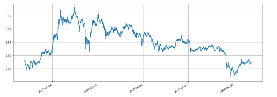
XTZ's market price has been in shock during the last 5 days, which is very suitable for grids.

We first backtest the effect of different holding positions on the profit return. The return backtested by the traditional backtest mechanism will definitely increase in proportion to the increase in holding positions.
e1 = Grid('XTZ',100,0.3,1000,maker_fee=-0.00002,taker_fee=0.0003)
print(e1.account['USDT'])
e2 = Grid('XTZ',1000,0.3,1000,maker_fee=-0.00002,taker_fee=0.0003)
print(e2.account['USDT'])
e3 = Grid('XTZ',10000,0.3,1000,maker_fee=-0.00002,taker_fee=0.0003)
print(e3.account['USDT'])
e4 = Grid('XTZ',100000,0.3,1000,maker_fee=-0.00002,taker_fee=0.0003)
print(e4.account['USDT'])
A total of four groups were backtested, the value of holding positions was 100, 1000, 10000, 100,000, and the total backtest time was 1.3s. The results are as follows:
{'realised_profit': 28.470993031132966, 'margin': 0.7982662957624465, 'unrealised_profit': 0.0104554474048441, 'total': 10000028.481448, 'leverage': 0.0, 'fee': -0.3430967859046398, 'maker_fee': -0.36980249726699727, 'taker_fee': 0.026705711362357405}
{'realised_profit': 275.63148945320177, 'margin': 14.346335829979132, 'unrealised_profit': 4.4382117331794045e-14, 'total': 10000275.631489, 'leverage': 0.0, 'fee': -3.3102045933457784, 'maker_fee': -3.5800688964477048, 'taker_fee': 0.2698643031019274}
{'realised_profit': 2693.8701498889504, 'margin': 67.70120400534114, 'unrealised_profit': 0.5735269329348516, 'total': 10002694.443677, 'leverage': 0.0001, 'fee': -33.984021415250744, 'maker_fee': -34.879233866850974, 'taker_fee': 0.8952124516001403}
{'realised_profit': 22610.231198585603, 'margin': 983.3853688758861, 'unrealised_profit': -20.529965947304365, 'total': 10022589.701233, 'leverage': 0.002, 'fee': -200.87094000385412, 'maker_fee': -261.5849078470078, 'taker_fee': 60.71396784315319}
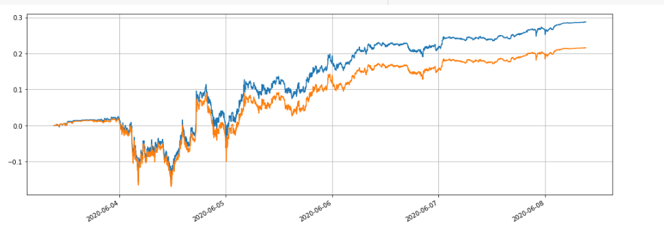
It can be seen that the final realized profits are 28.4%, 27.5%, 26.9% and 22.6% of the holding position value respectively. This is also in line with the actual situation. The greater the value of the holding position, the greater the value of the pending order, the more likely a partial transaction will occur, and the smaller the final realized gain relative to the amount of the pending order. The following chart is a comparison of the relative returns of the position value of 100 and 10000 respectively:

We can also backtest the impact of different parameters on backtest revenue, such as pending order density, sleep time, transaction fee, etc. Take the sleep time as an example, change it to 100ms, and compare the sleep time to 1000ms to see the profit return. The backtest results are as follows:
{'realised_profit': 29.079440803790423, 'margin': 0.7982662957624695, 'unrealised_profit': 0.0104554474048441, 'total': 10000029.089896, 'leverage': 0.0, 'fee': -0.3703702128662524, 'maker_fee': -0.37938946377435134, 'taker_fee': 0.009019250908098965}
earnings have increased a bit, because the strategy only sends a set of orders, some orders will not be able to execute fluctuating prices because they have no time to change, and the reduction of sleep time improves this problem. This also illustrates the importance of grid strategy for placing multiple sets of orders.
To sum up
This article innovatively proposes a new backtest system based on order flow, which can partially simulate the matching situation of pending orders, executing orders, partial executed orders, delays, etc., and partially reflects the impact of the amount of strategy funds on revenue. For high-frequency and hedging strategies, It has important reference value. High-precision backtest indicates the direction for strategy parameter optimization. It has also been verified for a long time. Moreover, the amount of data required for backtest is well controlled, and the backtest speed is also very fast.
