The collapse of FMEX has harmed many people, but it recently came up with a restart plan and formulated rules similar to the original mining to unlock their debt. For transaction mining, I have given an analysis article, https://www.fmz.com/bbs-topic/5834. At the same time, there is room for optimization in sorting mining. Although people should not step into the same pit twice, those who have financial claims on FMEX may want to give it a try, the specific real market strategies will also be released.
FMEX sort unlock rules
Define every 5 minutes in each day as a sorting unlocking cycle, and each cycle allocates 1/288 of the trading pair's sorting unlocking amount of the day. Within each cycle, a time point is randomly selected to take a snapshot image of the transaction on the pending orders of the trading orders, in which:
Buy 1 According to the proportion of the user's pending order amount, allocate 1/4 of the refund amount of the sorting unlock cycle
Sell 1 According to the proportion of the amount of the user's pending order, allocate 1/4 of the refund amount of the sorting unlock cycle
Buy 2 to Buy 5 of these four pending order layers, according to the proportion of the amount of the user's orders in each order, the allocation of the order unlocking cycle is divided into 1/40
Sell 2 to Sell 5 of these four pending order layers, according to the proportion of the amount of the user's orders in each order, the allocation of the order unlocking cycle is divided into 1/40
Buy 6 to Buy 10 of these five pending order layers, according to the proportion of the amount of the user's orders in each order, the allocation of the order unlocking cycle is divided into 1/50
Sell 5 to Sell 10 of these five pending order layers, according to the proportion of the amount of the user's orders in each order, the allocation of the order unlocking cycle is divided into 1/50
Buy 11 to Buy 15 of these five pending order layers, according to the proportion of the amount of the user's orders in each order, the allocation of the order unlocking cycle is divided into 1/100
Sell 5 to Sell 15 of these five pending order layers, according to the proportion of the amount of the user's orders in each order, the allocation of the order unlocking cycle is divided into 1/100
The total refund of a user's order unlocking in a certain trading pair on the same day is the sum of the amount of credits returned by the user's order unlocking of each cycle in the transaction.
Sorting unlock income
First, the total income of sorting and unlocking are:

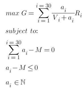
Where i represents one of the positions, and there are 30 positions on both sides, a is the amount of pending orders, R is the unlocked refund amount, and V is the total amount of existing orders.
Unlike transaction unlocking, there is no cost for pending orders. R here only considers the relative size, and does not need to consider the absolute amount of USDT pricing. If we determine the total amount of pending orders, the question becomes how to allocate the orders to different positions to maximize the profit G. Simply looking for the position with the smallest amount of pending orders and pending them all up is obviously not the optimal solution. As an example, the existing pending orders in three positions are all 10, and their R is the same. We set the total pending order amount to 30. If only one position is selected, the final total return is 0.75R. If each position is placed 10, the final return is 1.5R, which shows that sometimes the return from the spread of pending orders is better. So how to allocate funds?
Optimization of sorting unlock
In the end, our optimization goals and constraints are:

Where M is the total number of pending orders. This is a quadratic convex optimization problem that contains inequalities, satisfies the KTT condition, and is solved as an integer. Using the corresponding package and convex optimization solver should be able to directly get the results and return the optimal amount of pending orders for each position. But this is obviously not the answer we want, we need to simplify the problem and get specific solution steps.
Start with a simple example
Only two price layers are considered. The current pending orders are 10 and 20 (called the first and second layers, respectively), and their unlocked amount is R, and the total amount of strategy pending orders is 30. How to allocate The funds reach the maximum unlocked amount? This question seems simple, but it is difficult to draw a correct conclusion without calculation. Readers may wish to think about the answer first.
Plan 1:
Find the position of the smallest pending order, hang up all of them, the total return will be G=30/(30+10)=0.75R. This is also the easiest solution to think of.
Plan 2:
Each time it is allocated 1 yuan, and allocated to the place that can generate the greatest profit, that is, the position with the smallest amount of pending orders. Then the first yuan will be allocated to the first price layer, the amount of pending orders in the first price layer will become 10+1, and the second yuan will also be allocated to the first price layer... and so on, until the cumulative is assigned to the first price layer of 10 yuan, then you can Choose one at random. When the total pending orders in the first price layer exceed 20, the next price layer will be assigned to the second price layer. The final result is 20 yuan for the first price layer and 10 yuan for the second price layer. Their final pending orders are all 30. The total return G=20/30+10/30=R. This option is much better than option 1 and is also easy to calculate.
Plan 3:
You can set the first price layer to allocate a, and the second price layer is 30-a, then you can directly list the equation and derive it as 0 (the process is omitted, similar to the article of unlocking trading), calculate the final result, the formula is:

Bring in the rounding to find a=15. The total return G=15/25+15/35=1.0286R, which is better than Plan 2. Since it is directly derived from the formula, this is the optimal option, readers can check it.
The result may be different from everyone's expectations. plan 2 clearly shows that the allocation of each element is the optimal solution under the current situation. Why not the overall optimal solution? This situation is very common, and the local optimality is not necessarily the overall optimality, because before the allocation, the amount of pending orders has already been invested, and the overall efficiency needs to consider the sunk cost. Our goal for each step of optimization is to achieve the highest overall efficiency rather than the highest single return.
Specific optimization plan
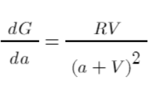
Finally, the actual feasible operation began, or to simplify the problem by allocating 1 yuan each time. First of all, measure the efficiency. The derivative can reflect the contribution of each copy of a to G. This contribution takes into account the cumulative cost, rather than the income of a single distribution. The larger the value, the greater the overall contribution to the final benefit. Obviously, according to the image of the function, a=1, from presence to absence, the efficiency is the highest, and then gradually decreases.

Similarly, taking the simple example above as an example, calculate their efficiency after allocating funds separately, and list the tables:
| Funds | 1 | 2 |
| 1 | 0.0826 | 0.0454 |
| 2 | 0.069 | 0.0413 |
| 3 | 0.0592 | 0.0378 |
| 4 | 0.051 | 0.0347 |
| 5 | 0.0444 | 0.032 |
| ... | ... | ... |
| 12 | 0.0207 | 0.0195 |
| 13 | 0.0189 | 0.0184 |
| 14 | 0.0174 | 0.0173 |
| 15 | 0.016 | 0.0163 |
| 16 | 0.0148 | 0.0154 |
| 17 | 0.0137 | 0.0146 |
| 18 | 0.0128 | 0.0139 |
According to the table, the first yuan is assigned to the first price layer, the second yuan is assigned to the first price layer... the fifth yuan is assigned to the second price layer... and so on, and finally assigned to the first price layer 15 yuan, the second price layer 15 Yuan is exactly the optimal solution we calculated according to the equation. Specific to the case of 30 price layers, the algorithm is the same, the specific steps are:
Check all price layers first, if
V=0, thena=1, no longer allocate excess funds.Allocate the total funds into
Nshares, and select a price layers to allocate at a time.Calculate the efficiency of each price layers =
RV/pow(a+V, 2),arepresents the accumulated funds allocated at this position + the funds allocated this time.Allocate funds to the most efficient price layers, and choose one randomly at the same efficiency.
Cycle 3-4 until the allocation of funds is completed.
If our total pending orders are large and the efficiency of each yuan allocation is too low, we can split the funds into 100 and allocate one each time. Since it is only a simple operation sorting, the efficiency of the algorithm is very high. Specific to the execution level, there is still room for optimization, such as dividing our orders into 100, so that each time you adjust, you only need to reassign the order and do not need to cancel it all. You can also set the R value yourself to give more weight to the far markets price. There are overlapping parts for sorting unlocking and pending order unlocking, which can be considered together, and so on.
From: FMEX trading unlocks the optimal order volume optimization Part 2 (fmz.com)
